Introduction to Pulse Control in Superconducting Qubits
$ \newcommand{\bra}[1]{\langle #1|} $ $ \newcommand{\ket}[1]{|#1\rangle} $ $ \newcommand{\braket}[2]{\langle #1|#2\rangle} $ $ \newcommand{\ketbra}[2]{| #1\rangle \langle #2|} $ $ \newcommand{\tr}{{\rm tr}} $ $ \newcommand{\i}{{\color{blue} i}} $ $ \newcommand{\Hil}{{\cal H}} $ $ \newcommand{\V}{{\cal V}} $ $ \newcommand{\bn}{{\bf n}} $
1. Introduction to Superconducting Qubits 
Superconducting qubits are one of the most extended technologies for quantum computer physical realization, some of the reasons fot this are the use of mesoscopic systems (macroscopic systems with quantum behaviour) and fast gate operations. Nevertheless, this kind of devices have many drawback which are yet to be solved: short coherence times, high sensitivity to noise, etc.
To understand how can we stablish the logic of a theoretical quantum computer on this kind of devices, it is necessary to study the physical implementation of superconducting qubits, gates, entanglement and measurements. For example, how do we define the computational basis of the qubit $\{\ket{0},\ket{1}\}$? How do we control the state of the qubit to apply a gate? How two qubits interact to achieve entanglement? How do we interact with the qubit to measure it?
1.1. Quantum Electromagnetic Circuits 
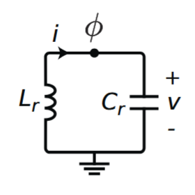
Before studying the superconducting qubit, we will briefly review how to describe a quantum electromagnetic field with Hamiltonians. As we said before, superconducting qubits are based o mesoscopic systems, these are man-made devices of macroscopic dimensions (contain a large number of atoms) with collective degrees of freedom that behave as a quantum system. One of the simplest is the superconducting LC circuit.
https://doi.org/10.1063/1.5089550
In its classical description, the energy of the system oscillates between the electrical energy of the capacitor C and the magnetic energy of the inductor L, equivalent to the exchange of kinetic and potential energy in a classical harmonic oscillator. The generic energy in each element can be derived from: $$E(t)=\int_{-\infty}^tV(t')I(t')\ \mathrm{d}t',$$ where $V$ and $I$ are the voltage and current measured in the element. To do the Hamiltonian characterization, we are going to define some generalized coordinates, the flux and charge: $$\begin{align*} \Phi(t)&=\int_{-\infty}^t V(t')\ \mathrm{d}t'\Rightarrow \dot{\Phi}(t)=\frac{\mathrm{d}\Phi}{\mathrm{d}t}(t)=V(t),\\ Q(t) &=\int_{-\infty}^t I(t')\ \mathrm{d}t'\Rightarrow \dot{Q}(t)=\frac{\mathrm{d}Q}{\mathrm{d}t}(t)=I(t). \end{align*}$$ Also, we have the following relations for the circuit's elements: $$\begin{align*} \text{Capacitor: }I_C&=C\frac{\mathrm{d}V_C}{\mathrm{d}t},\\ \text{Inductor: }V_L&=L\frac{\mathrm{d}I_L}{\mathrm{d}t}\Rightarrow I_L=\frac{1}{L}\int_{-\infty}^t V_L(t')\ \mathrm{d}t'=\frac{1}{L}\Phi(t). \end{align*}$$ Let's express the energy in each element as a function of the coordinate $\Phi$: $$\begin{align*} \text{Capacitor: }T_C &=\int_{-\infty}^tV_C(t')I_C(t')\ \mathrm{d}t'=C\int_{-\infty}^tV_C(t')\frac{\mathrm{d}V_C}{\mathrm{d}t'}(t')\ \mathrm{d}t\\ &=C\Bigl[V_C^2(t')\Bigl]_{\infty}^t-C\int_{-\infty}^tV_C(t')\frac{\mathrm{d}V_C}{\mathrm{d}t'}(t')\ \mathrm{d}t=\frac{1}{2}C\Bigl[V_C^2(t')\Bigl]_{\infty}^t=\frac{1}{2}C\Bigl[\dot{\Phi}(t)-\dot{\Phi}(-\infty)\Bigl]=\frac{1}{2}C\dot{\Phi}(t)-T_\text{C,offset},\\ \text{Inductor: }U_L &=\int_{-\infty}^tV_L(t')I_L(t')\ \mathrm{d}t'=\frac{1}{2}L\Bigl[I_L^2(t')\Bigl]_{\infty}^t=\frac{1}{2L}\Bigl[\Phi^2(t')\Bigl]_{\infty}^t=\frac{1}{2L}\Phi^2(t)-U_\text{L,offset}. \end{align*}$$ The Lagrangian of the system, setting the offset energies to zero, is: $$\mathcal{L}=T_C-U_L=\frac{1}{2}C\dot{\Phi}^2(t)-\frac{1}{2L}\Phi^2(t),$$ where we can define the momentum conjugate to the flux, the charge on the capacitor: $$Q=\frac{\mathrm{d}\mathcal{L}}{\mathrm{d}\dot{\Phi}}=C\dot{\Phi}.$$ The Hamiltonian of the system can be expressed as: $$H_\text{LC}=Q\dot{\Phi}-\mathcal{L}=\frac{1}{2}C\dot{\Phi}^2+\frac{1}{2L}\Phi=\frac{Q^2}{2C}+\frac{\Phi^2}{2L},$$ equivalent to a classical harmonic oscillator (CHO) with mass $m=C$ and resonant frequency $\omega=1/\sqrt{LC}$: $$H_{CHO}=\frac{P^2}{2m}+\frac{m\omega^2}{2}X^2.$$ The variables $\Phi$ and $Q$ are conjugates coordinates, and as such, they verify the Poisson bracket relation $\{\Phi,Q\}=1$. Considering $\hat{\Phi}$ and $\hat{Q}$ their promoted quantum operators, we have the commutation relation $[\hat{\Phi},\hat{Q}]=i\hbar$. The Hamiltonian of the quantum system is: $$H_\text{QLC}=\frac{\hat{Q}^2}{2C}+\frac{\hat{\Phi}^2}{2L}$$ It will be useful to define the following reduxed coordinates, later we will explain what their physical meaning is: $$\begin{align*} &\text{Reduxed flux: } \phi:=2\pi\hat{\Phi}/\Phi_0,\ \text{where $\Phi_0=h/(2e)$ is the quantum of superconducting magnetic flux};\\ &\text{Reduxed charge: } n:=\hat{Q}/2e, \end{align*}$$ that verify $[\phi,n]=i$. The Hamiltonian of the quantum system can be expressed as: $$H=4E_Cn^2+\frac{1}{2}E_L\phi^2,$$ where $E_C=e^2/(2C)$ and $E_L =(\Phi_0/2\pi)^2/L$. This Hamiltonian is equivalent to a quantum harmonic oscillator (QHO) with $\omega_r=\sqrt{8E_L E_C}/\hbar=1/\sqrt{LC}$: $$H=\hbar\omega_r\Bigl(a^\dagger a+\frac{1}{2}\Bigl).$$
1.2 Charge Superconducting Qubits: Transmons 
Considering the energy eigenstates of the quantum LC system (eigenstates of $a^\dagger a$), $\{\ket{n}\}_{n=0}^\infty$, we could define the computational basis on the two lowest energy levels, $\ket{0}$ and $\ket{1}$, and apply pulses of photons with the transition energy $\hbar\omega_r$ to excite or relax the system, thus having control over its state. The main problem of this configuration is its harmonicity, as all energy levels are equally spaced. This means that we have no control over which excitantion is going to produce from a photon of energy $\hbar\omega_r$. Fortunately, there is a similar kind of device that helps mitigate this problem: the Josephson qubit circuit.
https://doi.org/10.1063/1.5089550
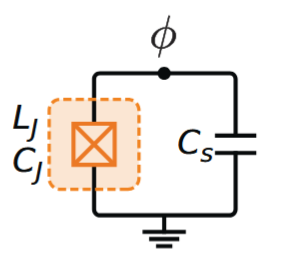
The Josephson junction is a set of two superconducting electrodes separated by a very thin oxide layer (insulator) that acts as a non-linear inductor (which breaks the harmonicity). The Josephson qubit circuit is composed of a Josephson junction in parallel to a capacitor, in a similar configurations as the LC circuit. At temperatures of order $\leq$ 100 mK, the electrons in the junction's sides condense in Cooper pairs, pair of electrons that behave as they are attracted to eachother due to interactions with the positive ions of the conductor in superconducting regime.
We can define the generalized flux of the junction $\phi$ as:
$$\phi(t)=\int_{-\infty}^t v_J(t')\ \mathrm{d}t',$$
being $v(t)$ a reduxed variable of the junction's voltage, similar to the inductor's flux from the LC circuit. But there is a different relation for the inductor's current:
$$\begin{align*}
&\text{Capacitance: }I_C=C\frac{\mathrm{d}V_C}{\mathrm{d}t}\ \text{(same as LC)},\\
&\text{Josephson junction: }I_J(t)=I_0\sin\phi(t),\ V_J=\frac{\hbar}{2e}\frac{\mathrm{d}\phi}{\mathrm{d}t}(t),
\end{align*}$$
where $I_0$ is the critical current of the junction.
With a similar procedure as before, we can obtain the energies in the capacitor and junction:
$$\begin{align*}
\text{Capacitance: }T_C &=\int_{-\infty}^tV_C(t')I_C(t')\ \mathrm{d}t'=C\int_{-\infty}^tV_C(t')\frac{\mathrm{d}V_C}{\mathrm{d}t'}(t')\ \mathrm{d}t\\
&=C\Bigl[V_C^2(t')\Bigl]_{\infty}^t-C\int_{-\infty}^tV_C(t')\frac{\mathrm{d}V_C}{\mathrm{d}t'}(t')\ \mathrm{d}t\\&=\frac{1}{2}C\Bigl[V_C^2(t')\Bigl]_{\infty}^t=\frac{1}{2}C\Bigl[\dot{\Phi}(t)-\dot{\Phi}(-\infty)\Bigl]=\frac{1}{2}C\dot{\Phi}(t),\\
\\
\text{Junction: }U_J &=\int_{-\infty}^tV_J(t')I_J(t')\ \mathrm{d}t'=\frac{\hbar I_0}{2e}\int_{-\infty}^t\frac{\mathrm{d}\phi}{\mathrm{d}t'}(t')\sin\phi(t')\ \mathrm{d}t'\\&=\frac{\hbar I_0}{2e}\Bigl[-\cos\phi(t')\Bigl]_{-\infty}^t=-\frac{\hbar I_0}{2e}\cos\phi(t)=-\frac{I_0\Phi_0}{2\pi}\cos\biggl(\frac{2\pi}{\Phi_0}\Phi(t)\biggl).
\end{align*}$$
The Lagrangian would be:
$$\mathcal{L}=T_C-U_L=\frac{1}{2}C\dot{\Phi}(t)+\frac{I_0\Phi_0}{2\pi}\cos\biggl(\frac{2\pi}{\Phi_0}\Phi(t)\biggl),$$
where the momentum conjugate is the same as before: $Q=C\dot{\Phi}$. The Hamiltonian for the Josephson qubit circuit can be expressed by the reduxed magnitudes $n=Q/(2e)$ and $\phi=2\pi\Phi/\Phi_0$:
$$\begin{align*}
H&=Q\dot{\Phi}-\mathcal{L}=\frac{1}{2}C\dot{\Phi} -\frac{I_0\Phi_0}{2\pi}\cos\biggl(\frac{2\pi}{\Phi_0}\Phi\biggl)\\
&=\frac{Q^2}{2C}-\frac{I_0\Phi_0}{2\pi}\cos\biggl(\frac{2\pi}{\Phi_0}\Phi\biggl)=\frac{4e^2}{2C}n^2-\frac{I_0\Phi_0}{2\pi}\cos\phi=4E_Cn^2-E_J\cos\phi,
\end{align*}$$
where $E_C=e^2/(2C)$, with $C$ the total capacitance of the circuit, and $E_J=I_0\Phi_0/(2\pi)$ the Josephson energy. As we can see, the Hamiltonian is very similar to the QHO, but with a cosinusoidal term for the position $\phi$ coordinate, which breaks de linearity. This term will introduce what is called anharmonicity, the energy levels of the oscillator will not be equally separeted.
Charge Superconducting Qubits
The Josephson circuit we have studied until now composes a familly of electromagnetic quantum circuits with different properties. The main difference between them is produced by the $E_J/E_C$ ratio of energies. The regime we are interested in, the one used in charge superconducting qubits, also called transmon, is $E_J\gg E_C$, which is less sensitive to charge noise. This can be achieved by incresing the capacitance of the capacitor. In this limit, the superconducting phase $\phi$ is small and we can approximate it by a non-linear potential well:
$$E_J\cos\phi = \frac{1}{2} E_J\phi^2 -\frac{1}{24}E_J\phi^4+\mathcal{O}(\phi^6).$$
This system can be model with a Duffing oscillator:
$$H=\hbar\omega_qa^\dagger a+\frac{\hbar\alpha}{2}a^\dagger a^\dagger a a,$$
where $\omega_q = (\sqrt{8E_J E_C}-E_C)/\hbar$ is the frequency for the $g\rightarrow e$ transition and $\alpha = \omega_q^{e\rightarrow f}-\omega_q^{g\rightarrow e}=-E_C<0$ is the anharmonicity of the transmon. As we are in the regime with $E_C\gg E_J$, we have that $|\alpha| \ll \omega_q$, which corresponds to a weekly anharmonic oscilator (AHO).
Generally, $|\alpha| \ll \omega_q$ lets us ommit the terms corresponding to the anharmonicity, leaving a simpler Hamiltonian:
$$H=-\hbar\omega_q\frac{\sigma_z}{2},$$
where $\sigma_z$ is the Pauli $Z$ operator for a 2D-Hilbert space, which is the physical description for a logical qubit. As we can see, we have encoded the computational basis $\{\ket{0},\ket{1}\}$ in the two lowest energy levels of the oscillator $\{\ket{g},\ket{e}\}$, leaving unaccesible higher energy levels.
2. Qubit Thermalization and Decoherence 
Until now, we have considered de qubit as an isolated system with some Hamiltonian $H=\hbar\omega_q\sigma_z/2$ that doesn't include any external influences. This is far from reality, as superconducting qubits rely on a very cold bath to initialize their state, at order of tens of mK. Here, we will study how the system behaves on a model for a simple photonic bath and how the thermalization process of the qubit works.
Let's consider a qubit in a isolated cavity with a bath of photons, the Hilbert space of the system is the tensor product of the system's space and the bath's space $\mathcal{H}=\mathcal{H}_S\otimes\mathcal{H}_E$, with $\dim(\mathcal{H}_E)\gg\dim(\mathcal{H}_S)=2$. Also, we will assume that the initial state of the system can be described by a separable density matrix:
$$\rho(0)=\rho_S(0)\otimes\rho_E(0).$$
The complete system will have a unitary time evolution given by some unitary operator $U(t)\in\text{Lin}(\mathcal{H})/ UU^\dagger=U^\dagger U=I$. The state in time $t\geq 0$ will be:
$$\rho(t)=U(t)\rho(0)U(t)^\dagger=U(t)\Bigl(\rho_S(0)\otimes\rho_E(0)\Bigl)U(t)^\dagger,$$
from where we can calculate the partial density matrix for the system, $\rho_S(t)=\text{Tr}_E\rho(t)$. Usually, for an isolated system, we can compute the time evolution by the Schrödinger equation:
$$\frac{\mathrm{d}\rho}{\mathrm{d}t}=-\frac{i}{\hbar}[H,\rho],$$
and that would be the case for $\rho=\rho_S\otimes\rho_E$ as, globally, is isolated. Unfortunately, the qubit subsystem, due to its interaction with the bath, won't evolve unitarely and this equation is not valid to represent the time evolution.
Time Evolution of a Qubit in a Photonic Bath
We can characterize the time evolution of the subsystem interacting with the environment using a more sophisticated expression, the Lindblad equation: $$\frac{\mathrm{d}\rho_S}{\mathrm{d}t}(t)=-\frac{i}{\hbar}[H,\rho_S(t)]+\sum_{k}\Bigl(L_k\rho_S(t)L_k^\dagger-\frac{1}{2}\{L_k^\dagger L_k,\rho_S(t)\}\Bigl),$$ where the first term corresponds to the Schrödinger time evolution and $\{L_k\}$ is a set of jump operators that model the environment, in our case the bath influence. Let's consider the following poissible interactions between the photons and the qubit:
- Excitation: the qubit absorbs a photon of energy $\hbar\omega_q$ with some probability $\Gamma_+$ and transitions from $\ket{0}$ to $\ket{1}$. The associated jump operator is: $$L_+=\sqrt{\Gamma_+}\begin{pmatrix}0 & 0\\ 1 & 0\end{pmatrix}.$$
- Relaxation: the qubit emits a photon of energy $\hbar\omega_q$ with some probability $\Gamma_-$ and transitions from $\ket{1}$ to $\ket{0}$. The associated jump operator is: $$L_-=\sqrt{\Gamma_-}\begin{pmatrix}0 & 1\\ 0 & 0\end{pmatrix}.$$
- Dephasing: the qubit changes its relative phase with some probability $\Gamma_\varphi$. The associated jump operator is: $$L_\varphi=\sqrt{\Gamma_\varphi}\begin{pmatrix}1 & 0\\ 0 & -1\end{pmatrix}.$$
Solving the Lindblad diffeential equation for this jump operator, we get the time evolution for a qubit in a photonic bath: $$\rho_S(t)=\begin{pmatrix} \rho_{S00}^{eq} +\Bigl(\rho_{S00}(0)-\rho_{S00}^{eq}\Bigl)e^{-t/T_1} & \rho_{S01}(0)e^{-t/T_2}e^{i\omega_q t}\\ \rho_{S10}(0)e^{-t/T_2}e^{-i\omega_q t} & \rho_{S11}^{eq} +\Bigl(\rho_{S11}(0)-\rho_{S11}^{eq}\Bigl)e^{-t/T_1} \end{pmatrix},$$ where $T_1=1/(\Gamma_++\Gamma_-)$, $T_2=1/\Bigl(\frac{\Gamma_++\Gamma_-}{2}+2\Gamma_\varphi\Bigl)$ are the decoherence times and $\rho_{S00}^{eq}=\Gamma_-T_1=\frac{\Gamma_-}{\Gamma_+ + \Gamma_-}$ and $\rho_{S11}^{eq}=\Gamma_+T_1=\frac{\Gamma_+}{\Gamma_+ + \Gamma_-}$ the equilibrium values when $t\rightarrow\infty$.
Expand for details
Let's use the Lindblad equation to compute $\rho_S(t)$: $$\begin{align*} \frac{\mathrm{d}\rho_S}{\mathrm{d}t}&=\begin{pmatrix}\dot{\rho_S}_{00} & \dot{\rho_S}_{01}\\ \dot{\rho_S}_{10} & \dot{\rho_S}_{11}\end{pmatrix},\\ \\ -\frac{i}{\hbar}[H,\rho_S(t)]&=-\frac{i}{\hbar}(H\rho_S-\rho_SH)=-i\omega_q\begin{pmatrix}0 & -\rho_{S01}\\ \rho_{S10} & 0\end{pmatrix},\\ \\ L_+^\dagger\rho_SL_+-\frac{1}{2}\{L_+^\dagger L_+,\rho_S\}&=\Gamma_+\begin{pmatrix}-\rho_{S00} & -\rho_{S01}/2\\ -\rho_{S10}/2 & \rho_{S00}\end{pmatrix},\\ \\ L_-^\dagger\rho_SL_--\frac{1}{2}\{L_-^\dagger L_-,\rho_S\}&=\Gamma_-\begin{pmatrix} \rho_{S11} & -\rho_{S01}/2\\ -\rho_{S10}/2 & -\rho_{S11} \end{pmatrix},\\ \\ L_\varphi^\dagger\rho_SL_\varphi-\frac{1}{2}\{L_\varphi^\dagger L_\varphi,\rho_S\}&=\Gamma_z\begin{pmatrix} 0 & -2\rho_{S01}\\ -2\rho_{S10} & 0 \end{pmatrix}. \end{align*}$$ We get the following diferential equation: $$\begin{align*} \dot{\rho_S}_{00} &= \Gamma_-\rho_{S11}-\Gamma_+\rho_{S00},\\ \\ \dot{\rho_S}_{11} &= \Gamma_+\rho_{S00}-\Gamma_-\rho_{S11},\\ \\ \dot{\rho_S}_{01} &= i\omega_q\rho_{S01}-\Gamma_+\rho_{S01}/2-\Gamma_-\rho_{S01}/2-2\Gamma_\varphi\rho_{S01}\\ &=\Bigl[i\omega_q-\Bigl(\frac{\Gamma_++\Gamma_-}{2}+2\Gamma_\varphi\Bigl)\Bigl]\rho_{S01}=-\Bigl(-i\omega_q+\frac{1}{T_2}\Bigl)\rho_{S01},\\ \\ \dot{\rho_S}_{10} &= -i\omega_q\rho_{S10}-\Gamma_+\rho_{S10}/2-\Gamma_-\rho_{S10}/2-2\Gamma_\varphi\rho_{S10}\\ &=\Bigl[-i\omega_q-\Bigl(\frac{\Gamma_++\Gamma_-}{2}+2\Gamma_\varphi\Bigl)\Bigl]\rho_{S10}=-\Bigl(i\omega_q+\frac{1}{T_2}\Bigl)\rho_{S10}, \end{align*}$$ where $T_2=1/\Bigl(\frac{\Gamma_++\Gamma_-}{2}+2\Gamma_\varphi\Bigl)$. As $\rho_S$ is a density matrix, $\text{Tr}\rho_S=\rho_{S00}+\rho_{S11}=1$, then $\rho_{S11}=1-\rho_{S00}$: $$\begin{align*} \dot{\rho_S}_{00} &= \Gamma_- -(\Gamma_++\Gamma_-)\rho_{S00}=\Gamma_- -\frac{1}{T_1}\rho_{S00},\\ \\ \dot{\rho_S}_{11} &= \Gamma_+ -(\Gamma_++\Gamma_-)\rho_{S11}= \Gamma_+ -\frac{1}{T_1}\rho_{S11}, \end{align*}$$ where $T_1=1/(\Gamma_++\Gamma_-)$. These differential equations are easly solvable: $$\begin{align*} \rho_{S00}(t)&=\rho_{S00}(0)e^{-t/T_1}+\Gamma_-T_1\Bigl(1-e^{-t/T_1}\Bigl)\\ &=\Gamma_-T_1 +\bigl(\rho_{S00}(0)-\Gamma_-T_1\bigl)e^{-t/T_1}=\rho_{S00}^{eq} +\Bigl(\rho_{S00}(0)-\rho_{S00}^{eq}\Bigl)e^{-t/T_1},\\ \\ \rho_{S11}(t)&=\rho_{S11}(0)e^{-t/T_1}+\Gamma_+T_1\Bigl(1-e^{-t/T_1}\Bigl)\\ &=\Gamma_+T_1 +\bigl(\rho_{S11}(0)-\Gamma_+T_1\bigl)e^{-t/T_1}=\rho_{S11}^{eq} +\Bigl(\rho_{S11}(0)-\rho_{S11}^{eq}\Bigl)e^{-t/T_1},\\ \\ \rho_{S01}(t)&=\rho_{S01}(0)e^{-\Bigl(-i\omega_q+\frac{1}{T_2}\Bigl)t}=\rho_{S01}(0)e^{-t/T_2}e^{i\omega_q t},\\ \\ \rho_{S10}(t)&=\rho_{S10}(0)e^{-\Bigl(i\omega_q+\frac{1}{T_2}\Bigl)t}=\rho_{S10}(0)e^{-t/T_2}e^{-i\omega_q t}. \end{align*}$$
When the elapsed time is long enough, the system evolves towards a partially mixed equilibrium state: $$\rho_S^{eq}=\rho_S(t\rightarrow\infty)=\begin{pmatrix} \rho_{S00}^{eq} &0\\ 0 & \rho_{S11}^{eq} \end{pmatrix},$$ with purity: $$\mathcal{P}(\rho_S^{eq})=\text{Tr}(\rho_S^{eq})^2=(\rho_{S00}^{eq})^2+(\rho_{S11}^{eq})^2=(\Gamma_-^2+\Gamma_+^2)T_1^2=\frac{\Gamma_-^2+\Gamma_+^2}{(\Gamma_-+\Gamma_+)^2}<1,\ \text{for any $\Gamma_-,\Gamma_+>0$},$$ that becomes maximally mixed for $\Gamma_+=\Gamma_-=\Gamma$: $$\mathcal{P}(\rho_S^{eq})=\frac{2\Gamma^2}{4\Gamma^2}=\frac{1}{2}.$$
Qubit Thermalization
It's been shown that, for a qubit in a thermal bath, the system evolution towards the equilibrium mixed state is characterize by some time parameters, that depend entirely on the interaction probabilities from the bath $\Gamma_i$:
- $T_1 = 1/(\Gamma_-+\Gamma_+)$ is the logitudinal relaxation time, which accounts for the time the qubit takes to decay to the equilibrium state.
- $T_2 = 1/(\frac{\Gamma_-+\Gamma_+}{2}+\Gamma_\varphi)=1/(\frac{1}{2T_1}+\frac{1}{T_\varphi})=2T_1T_\varphi/(2T_1+T_\varphi)$ is the transverse relaxation time.
This coefficients can be expressed in terms of rates:
- $\Gamma_1=\frac{1}{T_1}=\Gamma_-+\Gamma_+$ is the longitudinal relaxation rate, which depends on the total rate of the interaction with the bath (absortion and emission). Represents at which rate the qubit loses its current (in principle may be pure) state and evolves to a mixed equilibrium state.
- $\Gamma_\varphi$ is the pure dephasing rate, which describes the depolarization of the qubit on the XY-plane of the Bloch sphere.
- $\Gamma_2=\frac{1}{T_2}=\Gamma_1/2+\Gamma_\varphi$ is the transverse relaxation rate, which depends on the mean rate of interaction an the pure dephasing rate. Describes the loss of coherence of a superposition state like $\ket{+}=(\ket{0}+\ket{1})/\sqrt{2}$, which will be afected by the longitudinal decay but also by the dephasing.
For now, we've worked with these rates as some arbitrary parameters from the environment but, for a photonic bath, we can give them a specific form based on the Maxwell-Boltzmann statictics. Let's consider the rates of excitation and relaxation as a the following function of the bath's temperature $T$:
$$\begin{align*}
\Gamma_- &= \frac{\gamma\exp\Bigl(\frac{\hbar\omega_q}{2k_BT}\Bigl)}{\exp\Bigl(\frac{\hbar\omega_q}{2k_BT}\Bigl)+\exp\Bigl(-\frac{\hbar\omega_q}{2k_BT}\Bigl)},\\
\\
\Gamma_+ &= \frac{\gamma\exp\Bigl(-\frac{\hbar\omega_q}{2k_BT}\Bigl)}{\exp\Bigl(\frac{\hbar\omega_q}{2k_BT}\Bigl)+\exp\Bigl(-\frac{\hbar\omega_q}{2k_BT}\Bigl)}
\end{align*}$$
where $\gamma$ is some normalization constant. We have the following expressions for the rest of parameters:
$$\begin{align*}
\rho_{S00}^{\text{eq}}&=\frac{\exp\Bigl(\frac{\hbar\omega_q}{2k_BT}\Bigl)}{\exp\Bigl(\frac{\hbar\omega_q}{2k_BT}\Bigl)+\exp\Bigl(-\frac{\hbar\omega_q}{2k_BT}\Bigl)}=\frac{1}{Z}\exp\Bigl(\frac{\hbar\omega_q}{2k_BT}\Bigl),\\
\\
\rho_{S11}^{\text{eq}}&=\frac{\exp\Bigl(-\frac{\hbar\omega_q}{2k_BT}\Bigl)}{\exp\Bigl(\frac{\hbar\omega_q}{2k_BT}\Bigl)+\exp\Bigl(-\frac{\hbar\omega_q}{2k_BT}\Bigl)}=\frac{1}{Z}\exp\Bigl(-\frac{\hbar\omega_q}{2k_BT}\Bigl),
\end{align*}$$
with $Z=\exp\Bigl(\frac{\hbar\omega_q}{2k_BT}\Bigl)+\exp\Bigl(-\frac{\hbar\omega_q}{2k_BT}\Bigl)$ the partition function. We can see that the equilibrium corresponds to a thermal Gibbs state for the system at temperature $T$.
In summary, when we let a qubit evolve inside a thermal bath, starting from a pure state, the interaction with the environment photons will make the system decay towards some mixed Gibbs state, where the distribution will depend on the bath's temperature. At the same time, the qubit will change its phase periodically, as it evolves to equilibrium. Both of this processes are sources of noise called thermal decoherence, and its parameters ($T_1$, $T_2$...) are used to characterize the superconducting qubits coherence time, this is the average time the qubit will stay on some constructed state before decaying to the Gibbs state given by the bath's temperature.
Qubit State Initialization and Decoherence Time in Quantum Computing
We've seen that a qubit in a thermal bath will evolve to a Gibbs state, in some characterize time, during a process called thermalization. This is a useful tool to obtain approximately pure states, but also will limit our coherent operational time on the system. As we saw before, in the equilibrium, the probability of the energy eigenstates of the system will be:
$$\begin{align*}
P_0(T) & =\text{Tr}(\ket{0}\bra{0}\rho_S^\text{eq})= \rho_{S00}^\text{eq} = \frac{1}{Z}\exp\Bigl(\frac{\hbar\omega_q}{2k_BT}\Bigl),\\
\\
P_1(T) & =\text{Tr}(\ket{1}\bra{1}\rho_S^\text{eq})= \rho_{S11}^\text{eq} = \frac{1}{Z}\exp\Bigl(-\frac{\hbar\omega_q}{2k_BT}\Bigl).
\end{align*}$$
As the temperature gets lower, the average energy from the thermal fluctuations will get lower, given by $k_BT$. In the $k_BT\ll \hbar\omega_q$ regime, the average energy of the interactions won't be enough to excite the qubit, and so, it'll likely remain on the groundstate. We can see this on the Gibbs state probabilities for $T\rightarrow 0$:
$$\begin{align*}
P_0(T\rightarrow 0)&=\lim_{T\rightarrow 0}\frac{\exp\Bigl(\frac{\hbar\omega_q}{2k_BT}\Bigl)}{\exp\Bigl(\frac{\hbar\omega_q}{2k_BT}\Bigl)+\exp\Bigl(-\frac{\hbar\omega_q}{2k_BT}\Bigl)}=1,\\
\\
P_1(T\rightarrow 0)&=\lim_{T\rightarrow 0}\frac{\exp\Bigl(-\frac{\hbar\omega_q}{2k_BT}\Bigl)}{\exp\Bigl(\frac{\hbar\omega_q}{2k_BT}\Bigl)+\exp\Bigl(-\frac{\hbar\omega_q}{2k_BT}\Bigl)}=0.
\end{align*}$$
As a direct consequence, the lower the temperature the purer the Gibbs state is:
$$\begin{align*}
&\mathcal{P}(T)=(\rho_{S00}^\text{eq})^2 + (\rho_{S11}^\text{eq})^2=P_0^2(T)+P_1^2(T)\xrightarrow{T\rightarrow 0}1.
\end{align*}$$
From a practical point of view, we can put the transmon in a thermal bath at a very low temperature (usually in the order of 15-20 mK) and let the system thermalize to an almost pure state $\ket{0}$. From this moment, any unitary operations over the qubit's system will result in controlled almost-pure states, ignoring other noise factors. This is the main reason to stablish the groundstate $\ket{0}$ as the initialization for qubits in quantum circuits; when we are done running our operations, we just let the qubit decay again to the groundstate to continue with other operations.
While being a natural way of initializing the qubit, it also comes with a heavy burden, the decoherence. Like we saw before, any state will decay to the Gibbs state close to $\ket{0}$, this limits the time we can be operating on our qubit, as the decay will introduce a non-unitary evolution that we can't reverse, loosing the coherence of our state. For example, if we apply a X gate, the system will transition to an initially almost pure $\ket{1}$ but, given enough time, it'll evolve to some mixed state and any operations on top of it will not correspond to what we would expect from applying them to $\ket{1}$. For this reason, the parameters $T_1$ and $T_2$ of the qubit are very significant, as they give us an estimate of how much time we can operate on the qubit without loosing coherence, also called coherence time. Any group of gates that we want to apply on our qubit will need to take less than this coherence time in order to show consistent results with its theoretical operation, and so, we have a limitation on how deep a circuit can be.
3. Qubit Pulse Control 
Now that we've studied how a transmon qubit system is described, the next step is to learn how one can control its state. If we want to implement any algorithm used in Quantum Computing on real hardware, we need to understand how its most basic operations can be performed. In this section, we will take a look at how to drive the qubit to a desired state and how different quantum gates can be implemented by the use of microwave frequency pulses.
3.1. Quamtum Gates 
Quantum gates are a unitary operators on the qubits subespaces that evolve the system to an objective state. We can separate the between 1-qubit gates and 2-qubit gates, depending on how many qubits they are applied on but, as we will see, any gate can be expressed as a composition of a fixed set of them, even if they operate on more that 2 qubits.
Single Qubit Gates
These gates represent unitary operator over the 2-dimensional Hilbert space $\mathbb{C}^2$, this means that, given some qubit state $\ket{\psi}$ with $||\psi||=1$, the application of any gate $U$ will keep the state's norm, $||U\psi||=1$. It is very useful to express this gates by its matrix representation, as for any gate it exist some unitary matrix $U\in\mathcal{M}_{2\times 2}(\mathbb{C})$, that verifies $U^\dagger U=U^\dagger U = I_2$. Here we will list some of the most important ones:
- Gate $X=\sigma_x=\begin{pmatrix}
0 & 1\\
1 & 0
\end{pmatrix}$: performs a transition between the basis states, $X\ket{0}=\ket{1}$ and $X\ket{1}=\ket{0}$.
- Gate $Y=\sigma_y=\begin{pmatrix}
0 & -i\\
i & 0
\end{pmatrix}$: performs a transition between the basis states but with an added phase, $Y\ket{0}=-i\ket{1}$ and $Y\ket{1}=i\ket{0}$.
- Gate $Z=\sigma_z=\begin{pmatrix}
1 & 0\\
0 & 0
\end{pmatrix}$: changes the relative phase of the basis states, $Z\ket{0}=\ket{0}$ and $Z\ket{1}=-\ket{1}$.
- Hadamard gate $H=\frac{1}{\sqrt{2}}\begin{pmatrix}
1 & 1\\
1 & -1
\end{pmatrix}$: creates and destroys superposition of the basis states, $H\ket{0}=\frac{1}{\sqrt{2}}(\ket{0}+\ket{1})=\ket{+}$ and $H\ket{1}=\frac{1}{\sqrt{2}}(\ket{0}+-\ket{1})=\ket{-}$. It's used in many quantum algorithms to initialize the circuit in a equally distributed superposition of the computational basis.
- $\sqrt{X}$ or $SX=\frac{1}{\sqrt{2}}\begin{pmatrix}
1+i & 1-i\\
1-i & 1+i
\end{pmatrix}$: similar to the Hadamard gate, but its implementation with pulses is more efficient and it's in the basic gate-set of Qmio.
- Rotation $R_X(\theta)=e^{-i\theta X/2}=\cos(\theta/2)I_2-i\sin(\theta/2)X=\begin{pmatrix}
\cos(\theta/2) & -i\sin(\theta/2)\\
-i\sin(\theta/2) & \cos(\theta/2)
\end{pmatrix}$: performs a rotation on the x-axis of the Bloch sphere.
- Rotation $R_Y(\theta)=e^{-i\theta Y/2}=\cos(\theta/2)I_2-i\sin(\theta/2)Y=\begin{pmatrix}
\cos(\theta/2) & -\sin(\theta/2)\\
\sin(\theta/2) & \cos(\theta/2)
\end{pmatrix}$: performs a rotation on the y-axis of the Bloch sphere.
- Rotation $R_Z(\theta)=e^{-i\theta Z/2}=\cos(\theta/2)I_2-i\sin(\theta/2)Z=\begin{pmatrix} e^{-i\theta/2} & 0\\ 0 & e^{i\theta/2} \end{pmatrix}$: performs a rotation on the z-axis of the Bloch sphere.
Any 1-qubit gate can be decomposed on this rotations: $$U(\theta,\phi,\lambda)=R_Z(\phi)R_Y(\theta)R_Z(\lambda)=\begin{pmatrix} e^{-i(\phi+\lambda)/2}\cos(\theta/2) & -e^{-i(\phi-\lambda)/2}\sin(\theta/2)\\ e^{i(\phi-\lambda)/2}\sin(\theta/2) & e^{i(\phi+\lambda)/2}\cos(\theta/2) \end{pmatrix}.$$
Two Qubits Gates
Two qubits gates are unitary operators over the 4-dimensional Hilbert space $\mathbb{C}^4$. Some of them can be expressed as a tensor product of 1-qubit gates, like $Z\otimes Z$, that would apply a $Z$ gate on both qubits, but there are also gates that are not separable. Generally, this kind of gates will introduce entanglement between the qubits and, as such, are of great importance for quantum algorithm. Here we list some of the more relevant ones:
- $\text{CNOT}=\ket{0}\bra{0}\otimes I_2 + \ket{1}\ket{1}\otimes X$: applies an $X$ gate over a objective qubit only if the control qubit is in the state $\ket{1}$. It's used in most quantum algorithms to produce full-entanglement with the Hadamard gate.
- $\text{CZ}=\ket{0}\bra{0}\otimes I_2 + \ket{1}\ket{1}\otimes Z$: applies an $Z$ gate over a objective qubit only if the control qubit is in the state $\ket{1}$.
- $\text{ECR}=\frac{1}{\sqrt{2}}(I\otimes X - X\otimes Y)$: the Echoed Cross-Resonance gate is used to make full-entanglement in superconducting qubits. It's implementation with pulses is more efficient, and it's used in the basic gate-set of Qmio.
3.2. Single Qubit Pulse Driving 
The gates from before are some ideal representation of the operations we want to perform over the qubit, but it's real implementation is not direct for most cases and not general to every quantum device. Here we'll focus on the most usual pulse driving scheme and hardware capabilities.
https://doi.org/10.1063/1.5089550
Let's from now on make the (big) assumtion that our qubit is totally isolated and described by the Hamiltonian:
$$H_q=-\frac{\hbar\omega_q}{2}\sigma_z,$$
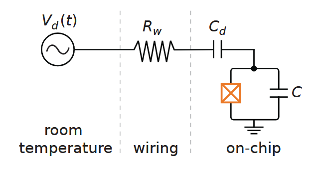
where $\omega_q$ is the qubit's resonance frequency and $\sigma_z=\begin{pmatrix}1 & 0\\ 0 & -1\end{pmatrix}$. To control its state, we will couple it to a microwave drive line, like the one in this figure:
(ñ: Poner esquema circuito)
The interaction with the driving line generated by some periodic potential signal $V_d(t)$ can be modeled by the following term:
$$H_d=-i\Omega V_d(t)(a-a^\dagger),$$
where $\Omega$ depends on the transmon's capacitances and the impedance of the circuit to ground, and $a$/$A^\dagger$ are the annhilation/creation operators for the qubit oscillator system. If we truncate this operators to the qubit Hilbert space (2-dimensional), we have the following expression in terms of Pauli operators:
$$\begin{align*}
a=\begin{pmatrix}
0 & 1\\
0 & 0
\end{pmatrix},\quad a^\dagger=\begin{pmatrix}
0 & 0\\
1 & 0
\end{pmatrix},\quad a-a^\dagger=\begin{pmatrix}
0 & 1\\
-1 & 0
\end{pmatrix};
\end{align*}$$
$$H_d=\Omega V_d(t)\sigma_y.$$
The Hamiltonian for the qubit coupled to the driving lane is:
$$H=H_0+H_d=-\frac{\hbar\omega_q}{2}\sigma_z+\Omega V_d(t)\sigma_y.$$
To study the effect of the driving on the qubit, we need to take into account the time evolution given by the qubit's system itself. As $H_0$ is time independent, the qubit's intrinsic time evolution will be characterized by the unitary operator:
$$U_{H_0}(t)=\exp(-iH_0t/\hbar)=\exp(i\omega_q t\sigma_z/2)=\cos(\omega_q t /2)I_2+i\sin(\omega_q t/2)\sigma_z=RZ(-\omega_q t),$$
which means that the qubit state will rotate over the z-axis of the Bloch sphere with frequency $\omega_q$. This evolution is only due to the qubit's oscillator system that depends only on the reasonance frequency $\omega_1$. So it'll make the next steps easier if we change the basis of our system, initially $\{\ket{0},\ket{1}\}$, to the one on the rotation frame:
$$\begin{align*}
\ket{0_{\text{rot}}}&=U_{H_0}(t)\ket{0}=e^{i\omega_q t/2}\ket{0},\\
\ket{1_{\text{rot}}}&=U_{H_0}(t)\ket{1}=e^{-i\omega_q t/2}\ket{1}.
\end{align*}$$
Note that this basis is still an eigenbasis for the system's Hamiltonian $H_0$:
$$\begin{align*}
H_0\ket{0_{\text{rot}}}&=e^{i\omega_q t/2}H_0\ket{0}=-\frac{\hbar\omega_q}{2} e^{i\omega_q t/2}\ket{0}=-\frac{\hbar\omega_q}{2}\ket{0_{\text{rot}}},\\
\\
H_0\ket{1_{\text{rot}}}&=e^{-i\omega_q t/2}H_0\ket{1}=\frac{\hbar\omega_q}{2} e^{-i\omega_q t/2}\ket{1}=\frac{\hbar\omega_q}{2}\ket{1_{\text{rot}}},
\end{align*}$$
where $\ket{0_{\text{rot}}}$ is the groundstate and $\ket{1_{\text{rot}}}$ the first excited state at any time $t$ and so, we can encode the computational basis on this frame, removing the intrinsic time evolution from the oscillator. This is called the rotation frame of the qubit, and helps simplify the next steps for the driving description. Given a generic state in some instant $t$:
$$\ket{\psi(t)}=U_{H_0}(t)\ket{\psi_0}=c_0e^{i\omega_q t/2}\ket{0}+ c_1e^{-i\omega_q t/2}\ket{1},$$
we can transform it to the rotating frame by applying the inverse unitary operator $U_{\text{rf}}=U_{H_0}^\dagger$:
$$\ket{\psi_{\text{rf}}}=U_{\text{rf}}\ket{\psi(t)}=c_0e^{i\omega_q t/2}U_{\text{rf}}\ket{0}+ c_1e^{-i\omega_q t/2}U_{\text{rf}}\ket{1}=c_0\ket{0}+ c_1\ket{1},$$
this is the state $\ket{\psi(t)}$ representation on the rotating frame basis $\{\ket{0_{\text{rot}}},\ket{1_{\text{rot}}}\}$.
Going back to our complete system with Hamiltonian $H$, we are going study the time-dependent Schrödinger equation for this $\ket{\psi_{\text{rf}}}=U_{\text{rf}}\ket{\psi(t)}$:
$$i\hbar\frac{\partial}{\partial t}\ket{\psi_{\text{rf}}}=\tilde{H}\ket{\psi_{\text{rf}}},$$
Expand for details
$$\begin{align*}i\hbar\frac{\partial}{\partial t}\ket{\psi_{\text{rf}}}&=i\hbar\frac{\partial}{\partial t}(U_{\text{rf}}\ket{\psi(t)})\\ &=i\hbar\Bigl(\frac{\partial}{\partial t}U_{\text{rf}}\Bigl)\ket{\psi(t)} +U_{\text{rf}}\Bigl[i\hbar \frac{\partial}{\partial t}\ket{\psi(t)}\Bigl]\\ &=i\hbar\dot{U}_{\text{rf}}\left(U_{\text{rf}}^\dagger\ket{\psi_{\text{rf}}}\right) + U_{\text{rf}}\left(H\ket{\psi(t)}\right)\\ &=i\hbar\dot{U}_{\text{rf}}U_{\text{rf}}^\dagger\ket{\psi_{\text{rf}}} + U_{\text{rf}}HU_{\text{rf}}^\dagger\ket{\psi_{\text{rf}}}=\Bigl(i\hbar\dot{U}_{\text{rf}}U_{\text{rf}}^\dagger+ U_{\text{rf}}HU_{\text{rf}}^\dagger\Bigl)\ket{\psi_{\text{rf}}}=\tilde{H}\ket{\psi_{\text{rf}}}. \end{align*}$$
which means that the time evolution on the rotating frame will be determined by the effective Hamiltonian: $$\tilde{H}=i\hbar\dot{U}_{\text{rf}}U_{\text{rf}}^\dagger+ U_{\text{rf}}HU_{\text{rf}}^\dagger,$$ where we can use $i\hbar\dot{U}_{\text{rf}}U_{\text{rf}}^\dagger+ U_{\text{rf}}H_0U_{\text{rf}}^\dagger=0$ to get the following expression: $$\tilde{H}=i\hbar\dot{U}_{\text{rf}}U_{\text{rf}}^\dagger+ U_{\text{rf}}(H_0+H_d)U_{\text{rf}}^\dagger=U_{\text{rf}}H_dU_{\text{rf}}^\dagger,$$ that only depends on the driving term of the original Hamiltonian. Expanding the operators, we end up with the effective Hamiltonian in the rotating frame for the qubit driving: $$\begin{align*} \tilde{H}&=U_{\text{rf}}H_dU_{\text{rf}}^\dagger=\Omega V_d(t) \bigl[\cos(\omega_q t)\sigma_y-\sin(\omega_q t)\sigma_x\bigl]. \end{align*}$$
It's time to give form to the potential $V_d(t)$ that generates the pulse. We're going to consider that the potential has a oscillatory component with a time-dependent amplitude: $$\begin{align*} V_d(t)&=V_0s(t)\sin(\omega_d t + \phi)\\ &=V_0s(t)\left[\cos(\phi)\sin(\omega_d t) + \sin(\phi)\cos(\omega_d t)\right], \end{align*}$$ where $V_0$ is the maximum pulse amplitude, $s(t)$ is the amplitude envelope function, $\omega_d$ is the frequency of the driving pulse and $\phi$ the initial phase. We can define the components of the pulse as: $$\begin{align*} \text{In-phase: }&\mathcal{I}=\cos(\phi),\\ \text{Out-of-phase: }&\mathcal{Q}=\sin(\phi),\\ \end{align*}$$ leaving the expression from before as: $$V_d(t)=V_0s(t)\left[\mathcal{I}\sin(\omega_d t) + \mathcal{Q}\cos(\omega_d t)\right].$$ Going back to the effective driving Hamiltonian: $$\begin{align*} \tilde{H}&=\Omega V_0s(t)\cdot\left[\mathcal{I}\sin(\omega_d t) + \mathcal{Q}\cos(\omega_d t)\right]\cdot\bigl[\cos(\omega_q t)\sigma_y-\sin(\omega_q t)\sigma_x\bigl]\\ &=\Omega V_0s(t)\cdot\left[\mathcal{I}\sin(\omega_d t)\cos(\omega_q t)\sigma_y + \mathcal{Q}\cos(\omega_d t)\cos(\omega_q t)\sigma_y - \mathcal{I}\sin(\omega_d t)\sin(\omega_q t)\sigma_x - \mathcal{Q}\cos(\omega_d t)\sin(\omega_q t)\sigma_x\right],\\ \end{align*}$$ we can use the rotating wave approximation (RWA) to remove the terms with higher frequencies, that only would introduce small oscillations around the global behaviour of the system. In this case, we are going to remove the oscillatory terms with frequency $\omega_d+\omega_q$, leaving only those with $\delta\omega=\omega_q-\omega_d$.
Expand for details
$$\begin{align*} 1.\ &\sin(\omega_dt)\cos(\omega t)=\cos(\omega_dt)\sin(\omega t)-\sin(\delta\omega t)=\sin((\omega_d+\omega)t)-\sin(\omega_dt)\cos(\omega t)-\sin(\delta\omega t)\\&\approx-\sin(\omega_dt)\cos(\omega t)-\sin(\delta\omega t) \Rightarrow\sin(\omega_dt)\cos(\omega t)=-\frac{1}{2}\sin(\delta\omega t);\\ \\ 2.\ &\cos(\omega_dt)\cos(\omega t)=-\sin(\omega_dt)\sin(\omega t)+\cos(\delta\omega t)=\cos((\omega_d+\omega)t)-\cos(\omega_dt)\cos(\omega t)+\cos(\delta\omega t)\\&\approx -\cos(\omega_dt)\cos(\omega t)+\cos(\delta\omega t)\Rightarrow\cos(\omega_dt)\cos(\omega t)=\frac{1}{2}\cos(\delta\omega t);\\ \\ 3.\ &\sin(\omega_dt)\sin(\omega t)=-\cos(\omega_dt)\cos(\omega t)+\cos(\delta\omega t)=\cos((\omega_d+\omega)t)-\sin(\omega_dt)\sin(\omega t)+\cos(\delta\omega t)\\&\approx-\sin(\omega_dt)\sin(\omega t)+\cos(\delta\omega t)\Rightarrow\sin(\omega_dt)\sin(\omega t)=\frac{1}{2}\cos(\delta\omega t);\\ \\ 4.\ &\cos(\omega_dt)\sin(\omega t)=\sin(\omega_dt)\cos(\omega t)+\sin(\delta\omega)=\sin((\omega_d+\omega)t)-\cos(\omega_dt)\sin(\omega t)+\sin(\delta\omega t)\\&\approx-\cos(\omega_dt)\sin(\omega t)+\sin(\delta\omega t)\Rightarrow\cos(\omega_dt)\sin(\omega t)=\frac{1}{2}\sin(\delta\omega t). \end{align*}$$
With this approximations, we have the following driving Hamiltonian: $$\begin{align*} \tilde{H}&=\Omega V_0s(t)\left(-\frac{\mathcal{I}}{2}\sin(\delta\omega t)\sigma_y + \frac{\mathcal{Q}}{2}\cos(\delta\omega t)\sigma_y - \frac{\mathcal{I}}{2}\cos(\delta\omega t)\sigma_x - \frac{\mathcal{Q}}{2}\sin(\delta\omega t)\sigma_x\right)\\ &=\frac{\Omega V_0}{2}s(t)\Bigl[-\left(\mathcal{I}\cos(\delta\omega t) + \mathcal{Q}\sin(\delta\omega t)\right)\sigma_x+\left(-\mathcal{I}\sin(\delta\omega t) + \mathcal{Q}\cos(\delta\omega t)\right)\sigma_y\Bigl], \end{align*}$$ and setting the drive frequency equal to the qubit's, $\delta\omega=\omega_q-\omega_d=0$, we get the general expression for the effective driving Hamiltonian in terms of the potential components and envelope function: $$\begin{align*} \tilde{H} &=\frac{\Omega V_0}{2}s(t)\Bigl(-\mathcal{I}\sigma_x+\mathcal{Q}\sigma_y\Bigl). \end{align*}$$
This is the expression from where we'll compute the time evolution of the system that performs the desired gate operations.
Rabi Oscillations and the $\pi$-pulse
Let's study first a simple case for the driving, consider $s(t)=1\ \forall t$ and $\phi=0$ $\left(\mathcal{I}=1,\ \mathcal{Q}=0\right)$:
$$\begin{align*}
\tilde{H}
&=-\frac{\Omega V_0}{2}\sigma_x,
\end{align*}$$
beacuse it's time independent, the unitary time evolution operator is:
$$\begin{align*}
U_{\phi=0}(t)=\exp\left(-i\tilde{H}t/\hbar\right)&=\exp\left(i\frac{\Omega V_0}{2\hbar}t\sigma_x\right)\\
\\
&=\exp\left(\frac{\Omega_R}{2}t\sigma_x\right)\\
\\
&=\cos\left(\Omega_Rt/2\right)I_2+i\sin\left(\Omega_Rt/2\right)\sigma_x\\
\\
&=\begin{pmatrix}
\cos\left(\Omega_Rt/2\right) & i\sin\left(\Omega_Rt/2\right)\\
i\sin\left(\Omega_Rt/2\right) & \cos\left(\Omega_Rt/2\right)
\end{pmatrix}=RX(-\Omega_R t),
\end{align*}$$
where we can see an oscillatory behaviour of frequency $\Omega_R=\Omega V_0/\hbar$. Let's assume that the qubit is initally in the pure qubit state $\ket{\psi_0}=a_0\ket{0}+a_1\ket{1}$, if we apply a pulse with the shape described before, the state of the system in some time arbitrary time $t$ is:
$$\begin{align*}
\ket{\psi(t)}&=U_{\phi=0}(t)\ket{\psi_0}\\
&=\left[a_0\cos\left(\Omega_Rt/2\right)+ia_1\sin\left(\Omega_Rt/2\right)\right]\ket{0}+\left[ia_0\sin\left(\Omega_Rt/2\right)+a_1\cos\left(\Omega_Rt/2\right)\right]\ket{1}.
\end{align*}$$
Let's observe how this time evolution affects each basis state:
$$\begin{align*}
P_0(t)&=|\bra{0}\ket{\psi(t)}|^2=|a_0|^2\cos^2\left(\Omega_Rt/2\right)+|a_1|^2\sin^2\left(\Omega_Rt/2\right),\\
\\
P_1(t)&=|\bra{1}\ket{\psi(t)}|^2=|a_0|^2\sin^2\left(\Omega_Rt/2\right)+|a_1|^2\cos^2\left(\Omega_Rt/2\right).
\end{align*}$$
(ñ: Insert Rabi oscillation graph)
This oscillatory behaviour between the two states under the driving pulse is called Rabi oscillation, and let's us control the state of the qubit. For example, let's consider an initial state $\ket{0}$ $\left(|a_0|^2 = 1,\ |a_1|^2 = 0\right)$, we can apply a $\pi$-pulse with duration $T_\pi=\pi/\Omega_R $ to promote it to $\ket{1}$:
$$U_{\phi=0}(T_\pi)=\begin{pmatrix}
0 & -i\\
-i & 0
\end{pmatrix}=-i\begin{pmatrix}
0 & 1\\
1 & 0
\end{pmatrix}=-i\sigma_x,$$
$$\begin{align*}\ket{\psi(T_\pi)}&=\left[a_0\cos\left(\pi/2\right)+ia_1\sin\left(\pi/2\right)\right]\ket{0}+\left[ia_0\sin\left(\pi/2\right)+a_1\cos\left(\pi/2\right)\right]\ket{1}=ia_1\ket{0}+ia_0\ket{1},
\end{align*}$$
$$\begin{align*}
P_0(T_\pi)&=|\bra{0}\ket{\psi(T_\pi)}|^2=|a_1|^2=0,\\
\\
P_1(T_\pi)&=|\bra{1}\ket{\psi(T_\pi)}|^2=|a_0|^2=1.
\end{align*}$$
If we apply again the same pulse on this new state, is easy to check that we get exactly the original state:
$$\ket{\psi(2T_\pi)}=a_0\ket{0}+a_1\ket{1}=\ket{0}.$$
This $\pi$-pulse is the pulse-level representation of a $X$ gate operation, leaving a global phase, in the ideal case ($p_0=1$):
$$\begin{align*}
U_{\phi=0}(T_\pi)\ket{0}&=i\ket{1}\equiv\ket{1}=X\ket{0},\\
\\
U_{\phi=0}(T_\pi)\ket{1}&=i\ket{0}\equiv\ket{0}=X\ket{1}.\\
\end{align*}$$
$SX$ Gate
The $\sqrt{X}$ gate, or $SX$ gate, is one of the basic operations directly implemented atb a pulse level in superdonducting devices like Qmio. It corresponds to a $\pi/2$ rotation along the $x$-axis in the Bloch sphere: $$SX=\frac{1}{2}\begin{pmatrix} 1+i & 1-i\\ 1-i & 1+i \end{pmatrix}=e^{i\pi/4}R_X(\pi/2),$$ which, for example, puts the system in superposition when applied to a initialized qubit. Let's see how to implement this gate at pulse-level, considering a constat envelope function, the driving Hamiltonian is again time-independent, but now we'll keep the initial phase $\phi$, therefore $\mathcal{I}$ and $\mathcal{Q}$, arbitrary: $$\hat{H}=\frac{\Omega V_0}{2}\Bigl(-\mathcal{I}\sigma_x+\mathcal{Q}\sigma_y\Bigl).$$ The time evolution for the system is given by the unitary operator: $$\begin{align*} U_\phi(t)&=\exp\left[-i\frac{\Omega V_0}{2\hbar}t\Bigl(-\mathcal{I}\sigma_x+\mathcal{Q}\sigma_y\Bigl)\right]=\exp\left[-i\frac{\Omega_R}{2}t\Bigl(-\mathcal{I}\sigma_x+\mathcal{Q}\sigma_y\Bigl)\right]\\ \\ &=\cos\left(\Omega_R t/2\right)I_2-i\sin\left(\Omega_R t/2\right)\left(-\mathcal{I}\sigma_x+\mathcal{Q}\sigma_y\right)\\ \\ &=\begin{pmatrix} \cos\left(\Omega_R t/2\right) & i(\mathcal{I}+i\mathcal{Q})\sin\left(\Omega_R t/2\right)\\ i(\mathcal{I}-i\mathcal{Q})\sin\left(\Omega_R t/2\right) & \cos\left(\Omega_R t/2\right) \end{pmatrix}\\ \\ &=\begin{pmatrix} \cos\left(\Omega_R t/2\right) & ie^{i\phi}\sin\left(\Omega_R t/2\right)\\ ie^{-i\phi}\sin\left(\Omega_R t/2\right) & \cos\left(\Omega_R t/2\right) \end{pmatrix}, \end{align*}$$ where we want to find some $T_{SX}$ and $\phi_{SX}$ such that $U_{\phi_{SX}}(T_{SX})\equiv SX$. It's easy to check that, for the parameters: $$\begin{align*} T_{SX}&=\frac{\pi}{2\Omega_R},\\ \phi_{SX}&=\pi, \end{align*}$$ which corresponds to a $\frac{\pi}{2}$-pulse with phase $\pi$ $\left(\mathcal{I}=-1,\ \mathcal{Q}=0\right)$. The unitary operator is not exactly $SX$ as described before: $$\begin{align*} U_{\phi_{SX}}(T_{SX}) &=\frac{1}{\sqrt{2}}\begin{pmatrix} 1 & -i\\ -i & 1 \end{pmatrix}=e^{-i\pi/4}\frac{1}{2}\begin{pmatrix} 1+i & 1-i\\ 1-i & 1+i \end{pmatrix}=e^{-i\pi/4}SX=R_X(\pi/2). \end{align*}$$ The pulse implementation performs the desired operation, but adds a global phase to the qubit's state, which is not a problem for 1-qubit gates. Nevertheless, for multiple qubit gates, we have to be aware of this global phase and check that it is being added to every quantum register during operations, in order to guarantee that non desired relative phases are being added between them.
Virtual $R_Z$ Gate
As we saw before, $R_X$ rotations correspond to pulses with an initial phase $\phi_X=\pi$: $$\begin{align*} U_{\pi}(t)=\begin{pmatrix} \cos\left(\Omega_R t/2\right) & -i\sin\left(\Omega_R t/2\right)\\ -i\sin\left(\Omega_R t/2\right) & \cos\left(\Omega_R t/2\right) \end{pmatrix}=R_X(\Omega_R t) \end{align*}.$$ In the same way, we can describe $R_Y$ rotations with the initial phase $\phi_Y=\pi/2$: $$U_{\pi/2}(t)=\begin{pmatrix} \cos\left(\Omega_R t/2\right) & -\sin\left(\Omega_R t/2\right)\\ \sin\left(\Omega_R t/2\right) & \cos\left(\Omega_R t/2\right) \end{pmatrix}=R_Y(\Omega_R t).$$ We can check that the $R_Y$ rotation can be decompose into $R_X$ and $R_Z$ rotations as follows: $$\begin{align*} R_Y(\theta)=R_Z(-\pi/2)R_X(\theta)R_Z(\pi/2). \end{align*}$$ which can be extended to rotations at any angle from the $x$-axis: $$\begin{align*}R_\beta(\theta)&=R_Z(-\beta)R_X(\theta)R_Z(\beta)=U_{\beta+\pi/2}(\theta/\Omega_R).\\ \end{align*}$$ The reason to call the $R_Z$ "virtual" is that we can apply it by just choosing an initial phase for the drive pulse of other gates, we do not need to implement it separately. As it is not a physical gate, it's considered to be perfect (fidelity of 1) and instantanous.
Universal Single Qubit Gate
The importance of the virtual $R_Z$ is even greater, as it'll let us implement any single qubit gate. We have that any unitary operator in $\mathbb{C}^2$ can be parametrized by a set of three angles $(\theta,\varphi,\lambda)$ ad follows:
$$\mathcal{U}(\theta,\varphi,\lambda)=\begin{pmatrix}
\cos(\theta/2) & -e^{i\lambda}\sin(\theta/2)\\
e^{i\varphi}\sin(\theta/2) & e^{i(\varphi+\lambda)}\cos(\theta/2)
\end{pmatrix}=R_Z\left(\varphi-\frac{\pi}{2}\right)R_X\left(\frac{\pi}{2}\right)R_Z\left(\pi-\theta\right)R_X\left(\frac{\pi}{2}\right)R_Z\left(\lambda-\frac{\pi}{2}\right),$$
so we can implement any single qubit gate a a combination of two calibrated pulses and the virtual $R_Z$. Let's see how the unitary pulse representation would be:
$$\begin{align*}
\mathcal{U}(\theta,\varphi,\lambda)&=R_Z\left(\varphi-\frac{\pi}{2}\right)U_{\pi/2}^{SX}R_Z\left(\pi-\theta\right)U_{\lambda}^{SX}\\
&=R_Z\left(\varphi-\frac{\pi}{2}\right)U_{\pi-\theta+\lambda}^{SX}U_{\lambda}^{SX},
\end{align*}$$
where the last $R_Z$ rotation doesn't change the proyective measurement results to the $\{\ket{0},\ket{1}\}$ basis. If this phase need's to be accounted for, we can simply let the qubit state rotate on it's frame to the desired angle.
For examle, we can parametrize the Hadamard gate as follows:
$$H=\mathcal{U}(\pi/2,0,\pi)=R_Z\left(\frac{\pi}{2}\right)U_{\pi/2}^{SX}U_{0}^{SX}$$
DRAG driving
There are several problems for using simple waveforms as constant or even gaussian, such as the possibility of exciting the $\ket{1}$ o $\ket{0}$ to higher energy levels or a dephasing effect that could change the resonance frequency of the qubit during the Rabi oscillation, both due to the interaction of the pulse that depends on the anharmonicity of the system. A very popular solution to mitigate this effects is the so called Derivative Reduction by Adiabatic Gate (DRAG). Originally, we assumed a very specific shape for the driving signal:
$$V_d(t)=V_0s(t)\left[\mathcal{I}\sin(\omega_d t) + \mathcal{Q}\cos(\omega_d t)\right],$$
where the envelope function $s(t)$ was the same for both in-phase and out-of-phase components. The idea is to use a new envelope shape $s'(t)$ that compensates the evolution to higher energy states, a general form for this function is:
$$s'(t)=\begin{cases}
s(t),\quad \text{on }\mathcal{I},\\
\lambda\dot{s}(t)/\alpha,\quad\text{on }\mathcal{Q},
\end{cases}$$
which means that the new generator potatial should look like:
$$V_d'(t)=V_0\left(s(t)\mathcal{I}\sin(\omega_d t) + \lambda\frac{\dot{s}(t)}{\alpha}\mathcal{Q}\cos(\omega_d t)\right),$$
where $\alpha$ is the anharmonicity and $\lambda\in[0,1]$ is some control parameter. For $\lambda = 0$ we recover the no-DRAG pulse, for $\lambda=0.5$ we optimally reduce the dephasing and for $\lambda=1$ we optimally reduce the leakage error to higher energy states. The problem is that we can't directly apply gates like this (only those of the original $s(t)$ shape), so we need to find a way to efficiently implement them by discretization.
For a gaussian waveform with duration $T$, standard deviation $\sigma$ and amplitude $A$:
$$\begin{align*} s(t)&=\frac{1}{\sqrt{2\pi\sigma^2}}\exp\left(-\frac{1}{2}\frac{(t-T/2)^2}{\sigma^2}\right),\\ s'(t)&=\frac{t}{\sqrt{2\pi\sigma^2}\sigma^2}\exp\left(-\frac{1}{2}\frac{(t-T/2)^2}{\sigma^2}\right)=\frac{t}{\sigma^2}s(t), \end{align*}$$
then, the new driving potential is: $$V_d'(t)=V_0s(t)\left(\mathcal{I}\sin(\omega_d t) + \lambda\frac{s(t)}{\alpha\sigma^2}\mathcal{Q}\cos(\omega_d t)\right),$$
3.3. Two Qubits Pulse Driving 
On charge superconducting qubits like Qmio, the most common two-qubit gate implementation is performed by an appropiate multi-qubit pulse driving, which implements the cross-resonance (CR) gate, or the more sophisticated version, the echoed-CR (ECR). Although other methods exist for flux-tunable qubits, here we'll focus on the first ones, in order to understand what Qmio physically implements when we call any multi-qubit gate.
Two-qubit coupling
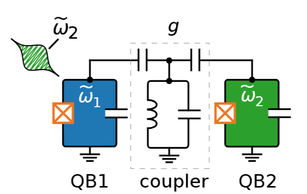
To apply a two-qubit gate, we need to study the effects of the multi-pulse drive on the qubit-qubit coupled system. Let's first consider two independent in-phase ($\phi=0$) drivings on the composite system (left qubit 1, right qubit 2): $$ \begin{align*} H_{d,1}&=-\frac{\Omega}{2}V_{d,1}(t)\ \sigma_x\otimes I,\\ \\ H_{d,2}&=-\frac{\Omega}{2}V_{d,2}(t)\ I\otimes\sigma_x. \end{align*} $$ Now, we'll add the coupling terms and perform a Schieffier-Wolff transformation to the dressed state frame, assuming that the coupling coefficient is much smaller than the two qubit's resonance frequency difference: $$ \begin{align*} H_{d,1}&=\Omega_c V_{d,1}(t)\ \left(\sigma_x\otimes I + \nu^-_1 I\otimes\sigma_x + \mu_1^-\sigma_z\otimes\sigma_x\right),\\ \\ H_{d,2}&=\Omega_c V_{d,2}(t)\ \left( I\otimes\sigma_x + \nu^+_2 \sigma_x\otimes I + \mu_2^+\sigma_x\otimes\sigma_z\right). \end{align*} $$
https://doi.org/10.1063/1.5089550
Let's consider that qubit 1 it's our control and 2 the target, the cross-resonance pulse is achieved by driving the control qubit with the target qubit's resonance frequency. In the drive expression for qubit 1, we will assume the usual in-resonance driving term is mitigated due to the detuning, the resulting expression shows a driving of the target qubit that depends on the control qubit state: $$\begin{align*} H_{d,1}&=\Omega_c V_{d,1}(t)\ \left(\nu^-_1 I+ \mu_1^-\sigma_z\right)\otimes\sigma_x. \end{align*}$$
This means that, when we drive the control qubit with the target's frequency, we produce a Rabi oscillation on the target that depends on the control's state.
4. References 
Krantz, P., Kjaergaard, M., Yan, F., Orlando, T. P., Gustavsson, S., Oliver, W. D. (2019) A quantum engineer's guide to superconducting qubits. Appl. Phys. Rev. 1 June 2019; 6 (2): 021318. doi: https://doi.org/10.1063/1.5089550
Vool, U., Devoret, M. (2017) Introduction to quantum electromagnetic circuits. Int. J. Circ. Theor. Appl., 45: 897–934. doi: https://doi.org/10.1002/cta.2359.
Lagemann, H. (2023). Real-time simulations of transmon systems with time-dependent Hamiltonian models. doi: https://doi.org/10.18154/RWTH-2023-02693.
Chen, Z. (2018). Metrology of Quantum Control and Measurement in Superconducting Qubits. UC Santa Barbara. ProQuest ID: Chen_ucsb_0035D_13771. Merritt ID: ark:/13030/m50p5xxf. Retrieved from https://escholarship.org/uc/item/0g29b4p0
J. Mas, Introduction to Quantum Simulation 2025/26 course notes, Master in Quantum Information Science and Technologies.